Technology & Methodology

Every ALKANE module draws on one thermodynamic engine, and every method built on it is named, sourced and checked against published reference data on Validation & Verification.

The equation of state

ALKANE solves phase behaviour, density and vapour–liquid equilibrium across the suite with the Peng-Robinson (1976) equation of state:

P = \frac{RT}{V-b} - \frac{a\alpha(T)}{V(V+b)+b(V-b)}

From composition, pressure and temperature, the engine resolves phase state, density and equilibrium K-values. Every module that depends on phase behaviour uses this same engine rather than an approximation of its own: phase envelope tracing, JT expansion, blowdown, orifice metering fluid properties, compressor discharge conditions and line pack bubble points.

Mixture behaviour depends on the binary interaction parameters as much as on the equation of state. ALKANE applies them through quadratic van der Waals mixing rules. For contaminant pairs (CO2, H2S and N2 against hydrocarbons, aromatics and one another), ALKANE uses Fateen, Khalil & Elnabawy (2013) where that paper covers the pair, and checks the remainder against an independent reference implementation. Hydrocarbon–hydrocarbon pairs use a correlation that increases with the separation between components. Analytical methods are used throughout for numerical stability and convergence.

Each problem then uses the method it requires:

Michelsen tangent-plane-distance analysis, to establish whether a phase split is thermodynamically real.
Arc-length continuation, to trace phase envelopes.
van der Waals-Platteeuw statistical thermodynamics, for hydrate equilibrium.
UV- and PS-flash formulations, for depressurisation, where a rigid vessel losing mass is governed by fixed volume and internal energy rather than a fixed expansion exponent.

Standards implemented

Peng-Robinson EOS
ISO 6976
GPA 2172
ISO 5167
AGA-3
IEC 60534
ISA-75.01.01
ASME B36.10M
API RP 14E
NIST ITS-90

These are the standards the calculations are implemented against. Naming them does not imply certification of the software.

Every method in the suite

Forty-six named methods, grouped by the part of the problem each one solves. Literature-sourced methods carry their citation; methods developed in-house are identified as such. Where a method is fitted to a particular fluid or range, or deliberately stops short of a calculation, its scope is stated with it.

Phase behaviour and thermodynamics10

Peng-Robinson equation of state
Compressibility, density, fugacity and caloric properties for every fluid the suite handles.
$P = \frac{RT}{V-b} - \frac{a(T)}{V(V+b)+b(V-b)}$
$a_i(T) = 0.45723553\,\frac{R^2 T_{c,i}^2}{P_{c,i}}\,\alpha_i(T), \qquad b_i = 0.07779607\,\frac{R\,T_{c,i}}{P_{c,i}}$
$\alpha_i = \left[1+\kappa_i\left(1-\sqrt{T/T_{c,i}}\right)\right]^2, \qquad \kappa_i = 0.37464 + 1.54226\,\omega_i - 0.26992\,\omega_i^2$
$Z^3 - (1-B)Z^2 + (A-3B^2-2B)Z - (AB-B^2-B^3) = 0, \qquad A = \frac{a\,P}{(RT)^2},\; B = \frac{b\,P}{RT}$
$\ln\varphi_i = \frac{b_i}{b_m}(Z-1) - \ln(Z-B) - \frac{A}{2\sqrt{2}\,B}\left[\frac{2\sum_j x_j a_{ij}}{a_m} - \frac{b_i}{b_m}\right]\ln\frac{Z+(1+\sqrt{2})B}{Z+(1-\sqrt{2})B}$
$a_{ij} = \sqrt{a_i a_j}\,(1-k_{ij})$
where $P$ is pressure, $T$ temperature, $V$ molar volume, $R$ the universal gas constant, $T_c$ and $P_c$ the critical temperature and pressure, $\omega$ the acentric factor and $Z$ the compressibility factor, solved analytically as the roots of the cubic. $\varphi_i$ is the fugacity coefficient of component $i$ in the mixture, with $a_{ij}$ as defined by the mixing rules.
Peng-Robinson cubic EOS
Quadratic van der Waals mixing rules with binary interaction parameters
Combines pure-component EOS parameters into mixture parameters, using a $k_{ij}$ matrix to resolve molecular asymmetry between dissimilar pairs.
$a_m = \sum_i \sum_j x_i x_j \sqrt{a_i a_j}\,(1-k_{ij}), \qquad b_m = \sum_i x_i b_i$
where $x$ is mole fraction, $a$ and $b$ the pure-component Peng-Robinson parameters and $k_{ij}$ the binary interaction parameter for the pair $i$ – $j$ .
Quadratic van der Waals mixing rules
Michelsen tangent plane distance stability analysis
Determines whether a feed is single-phase or will split into two phases.
$d_i = \ln z_i + \ln\varphi_i(\mathbf{z})$
$\ln W_i = d_i - \ln\varphi_i(\mathbf{W})$
$\text{feed unstable (phase split) if}\quad \sum_i W_i > 1$
where $\mathbf{z}$ is the feed composition and $\mathbf{W}$ the trial-phase mole numbers.
Michelsen's Tangent Plane Distance (TPD) analysis (1982)
Wilson correlation K-value estimate
Provides the starting estimate for the two-phase flash, with a full stability analysis applied where the estimate does not converge.
$K_i = \frac{P_{c,i}}{P}\exp\left[5.373\,(1+\omega_i)\left(1-\frac{T_{c,i}}{T}\right)\right]$
$\sum_i \frac{z_i (K_i-1)}{1+\beta(K_i-1)} = 0, \qquad x_i = \frac{z_i}{1+\beta(K_i-1)}, \quad y_i = K_i x_i$
where $K_i$ is the equilibrium ratio $y_i/x_i$ , $\beta$ the vapour fraction from the Rachford-Rice equation, and $x$ , $y$ the liquid and vapour compositions.
Wilson correlation
Arc-length continuation envelope tracing
Traces the full P-T phase envelope as independently discovered segments, so a wide-boiling composition with a genuine gap in its saturation curve is reported as a gap rather than bridged onto an unrelated root.
Arc-length continuation
Exact analytical EOS and fugacity derivatives
Closed-form derivatives of the equation of state, used for numerical stability and convergence in the phase-equilibrium solvers.
Developed in-house.
Pedersen & Fredenslund CS1 corresponding-states viscosity
Mixture viscosity across the gas, dense-gas and liquid range, with methane as the reference fluid.
Pedersen & Fredenslund (1987) "CS1" one-reference-fluid corresponding-states viscosity model
Kell (1975) pure-water density
Liquid water density from the Kell rational fit in temperature, with a linear compressibility correction, checked against IAPWS-95 across its range.
Kell (1975), J. Chem. Eng. Data 20(1), 97-105
Vogel-Fulcher-Tammann water viscosity fit
Liquid water viscosity as an exponential fit in temperature.
Vogel (Vogel-Fulcher-Tammann) exponential fit
Kay's Rule pseudo-critical properties
Mole-fraction-weighted pseudo-critical temperature and pressure for a mixture, used as a shared foundation wherever a module needs a mixture critical property rather than a full EOS solve.
Kay's Rule

Hydrates and Joule-Thomson expansion8

van der Waals-Platteeuw solid-solution theory
Multi-component gas hydrate equilibrium, evaluating Structure I and Structure II lattices independently and reporting which one forms.
$\frac{\Delta\mu_w^{H}}{RT} = \sum_m \nu_m \ln\left(1+\sum_j C_{mj}\,f_j\right)$
$\frac{\Delta\mu_w^{L}}{RT} = \frac{\Delta\mu_w^{0}}{RT_0} - \frac{\Delta h_w^{0}}{R}\left(\frac{1}{T}-\frac{1}{T_0}\right) - \frac{\Delta C_p}{R}\left[\ln\frac{T}{T_0} - \frac{T-T_0}{T}\right] + \frac{\Delta V_w\,P}{RT} - \ln a_w$
$\Delta\mu_w^{H}(T,P) = \Delta\mu_w^{L}(T,P)$
where $\nu_m$ is the number of cavities of type $m$ per water molecule, $C_{mj}$ the Langmuir constant of guest $j$ in cavity $m$ , $f_j$ its gas-phase fugacity from the Peng-Robinson engine, $\Delta\mu_w^0$ , $\Delta h_w^0$ , $\Delta V_w$ and $\Delta C_p$ the reference-state properties of Munck et al., and $a_w$ the water activity. Solved for temperature at the given pressure, separately for Structure I and Structure II.
van der Waals-Platteeuw statistical solid-solution model
Parrish-Prausnitz / Munck Langmuir coefficients
The classical fitted temperature-dependent Langmuir constant, used as the default hydrate model.
$C_{mj}(T) = \frac{A_{mj}}{T}\exp\left(\frac{B_{mj}}{T}\right)$
where $A_{mj}$ and $B_{mj}$ are fitted constants for guest $j$ in cavity $m$ .
Parrish-Prausnitz / Munck coefficients
Munck reference-state chemical potentials
Empty-hydrate-lattice chemical potential and enthalpy differences relative to pure liquid water, for Structure I and Structure II.
Munck et al. (1988) standard-state properties
Bukacek water content correlation
Saturated water content of a gas stream as a function of temperature and pressure.
Bukacek correlation
Joule-Thomson coefficient from the equation of state
Computes the Joule-Thomson coefficient straight from the equation of state rather than from a tabulated approximation, giving the temperature change per unit pressure drop at constant enthalpy. The derivation is verified numerically against an independent method.
$\mu_{JT} = \left(\frac{\partial T}{\partial P}\right)_H = \frac{T\left(\partial V/\partial T\right)_P - V}{C_p} = \frac{R\,T^2}{C_p\,P}\left(\frac{\partial Z}{\partial T}\right)_P$
where $C_p$ is the real-fluid isobaric heat capacity from the equation of state and $(\partial Z/\partial T)_P$ is evaluated analytically.
Developed in-house.
Marching isenthalpic expansion solver
Follows an isenthalpic pressure drop along its full path, resolving it through the two-phase region rather than solving only the endpoint.
Developed in-house.
Water activity model for inhibited and saline systems
Predicts how methanol, MEG and dissolved salts lower the activity of water, which is what suppresses the temperature at which hydrate will form. Reproduces the Hammerschmidt correlation closely across its range; inhibited results are indicative, not a dosing calculation.
Developed in-house.
Aqueous freezing point depression
Reports where the aqueous phase of the actual stream freezes, accounting for salinity and injected inhibitor, instead of asserting the pure-water ice point.
Developed in-house.

Depressurisation5

UV-flash solver
Solves equilibrium temperature, pressure and phase split at fixed molar volume and fixed internal energy — the operation a rigid vessel losing mass and gaining ambient heat actually requires at each timestep.
$U_{k+1} = U_k - h_{out}\,\Delta n + Q\,\Delta t$
$\text{find } (T,P)\ \text{such that}\quad v(T,P) = \frac{V}{n_{k+1}}, \qquad u(T,P) = \frac{U_{k+1}}{n_{k+1}}$
where $U$ is the vessel internal energy, $h_{out}$ the enthalpy of the leaving stream, $\Delta n$ the moles discharged in the step and $Q$ the ambient heat input; $v$ and $u$ are the molar volume and internal energy of the equilibrium mixture, two-phase where the stability test requires.
Brent, Algorithms for Minimization without Derivatives (root-finding within the solver)
PS-flash solver
Solves the downstream state of a fixed composition expanded at constant molar entropy to a given pressure, accounting for any phase change along the way rather than applying a fixed isentropic exponent.
$\text{find } T \text{ at fixed } P \text{ such that}\quad s(T,P) = s_{target}, \qquad s = \beta\,s_V + (1-\beta)\,s_L$
where $s$ is molar entropy and $\beta$ the vapour fraction where the outlet is two-phase.
Developed in-house.
Homogeneous equilibrium discharge model
Discharge mass flux by direct integration of the real isentropic expansion path, which — unlike the analytical choked-flow equation — can serve a liquid draw as well as a vapour one.
$s(T_{th}, P_{th}) = s_0, \qquad G(P_{th}) = \rho_{th}\sqrt{2\,(h_0 - h_{th})}$
$G_{choked} = \max_{P_{th}} G(P_{th})$
where $G$ is the discharge mass flux, subscript $0$ the vessel state and $th$ a trial throat state reached by isentropic flash. If $G$ rises monotonically to the back pressure, the flow is subcritical and $G$ at the back pressure is used.
Homogeneous Equilibrium Model (HEM)
Two-zone vessel depressurisation with liquid heel
A mathematical model of a depressurising vessel as two zones, liquid and vapour, at a common pressure but separate temperatures. Built on conservation of energy and mass, it predicts heat flux through the wall and insulation, boil-off, phase change and discharge from either draw point.
Developed in-house.
Entropy conservation check
Checks across a depressurisation run that the integration conserves entropy, as it must for an adiabatic rigid vessel under the equilibrium assumption.
Developed in-house.

Heat transfer5

Cooper pool-boiling correlation
Nucleate pool-boiling heat transfer from a reduced-pressure correlation, returning no value outside its validated reduced-pressure range rather than extrapolating.
M.G. Cooper, "Heat Flow Rates in Saturated Nucleate Pool Boiling"
A pure-fluid correlation, applied here to mixtures.
Churchill-Chu natural convection correlation
Natural-convection film coefficient for a vertical surface across laminar and turbulent regimes.
Churchill & Chu, Int. J. Heat Mass Transfer 18 (1975)
Horizontal-plate natural convection correlations
Natural convection from horizontal surfaces, where the vertical-surface correlation would mis-apply because the boundary layer overturns differently.
Incropera & DeWitt, Fundamentals of Heat and Mass Transfer; correlations originating with McAdams
Chung-Ajlan-Lee-Starling thermal conductivity
Thermal conductivity derived from the fluid properties the equation of state already provides, rather than from a separately fitted correlation.
Chung, Ajlan, Lee & Starling, "Generalized Multiparameter Correlation"
Overall heat transfer coefficient model
Series resistance across wall and optional insulation to ambient, giving a geometry-agnostic Q = UA·ΔT for both vessels and pipelines, so a depressurisation need not assume perfect adiabatic behaviour.
Developed in-house.

Metering and gas quality7

ISO 5167 orifice metering with the Reader-Harris/Gallagher discharge coefficient
Differential-pressure flow measurement across an orifice plate, solving for flow rate, bore or pipe diameter, with expansibility and isentropic exponent handled explicitly and out-of-range geometry surfaced as warnings.
$C = 0.5961 + 0.0261\beta^2 - 0.216\beta^8 + 0.000521\left(\frac{10^6\beta}{Re_D}\right)^{0.7} + (0.0188+0.0063A)\,\beta^{3.5}\left(\frac{10^6}{Re_D}\right)^{0.3}$
$\quad + \left(0.043 + 0.080e^{-10L_1} - 0.123e^{-7L_1}\right)(1-0.11A)\frac{\beta^4}{1-\beta^4} - 0.031\left(M_2' - 0.8M_2'^{1.1}\right)\beta^{1.3}$
$A = \left(\frac{19000\,\beta}{Re_D}\right)^{0.8}, \qquad M_2' = \frac{2L_2'}{1-\beta}$
$\varepsilon = 1 - \left(0.351 + 0.256\beta^4 + 0.93\beta^8\right)\left[1-\left(\frac{p_2}{p_1}\right)^{1/\kappa}\right]$
$q_m = \frac{C}{\sqrt{1-\beta^4}}\,\varepsilon\,\frac{\pi}{4}d^2\sqrt{2\,\rho_1\,\Delta p}, \qquad Re_D = \frac{4\,q_m}{\pi\,\mu\,D}$
where $\beta = d/D$ , $L_1$ and $L_2'$ are the tapping positions, $\kappa$ the isentropic exponent, $\rho_1$ the upstream density and $\mu$ the viscosity. $C$ and $Re_D$ are iterated together to convergence; the standard's small-bore term is added below its pipe-size threshold.
ISO 5167; Reader-Harris/Gallagher discharge coefficient equation
AGA-3 differential pressure metering
The AGA-3 treatment of orifice metering, offered alongside ISO 5167.
AGA Report No. 3
ISO 6976 / GPA 2172 heating value and combustion metrics
Calorific value, relative density, Wobbe index and related combustion metrics, on both dry and water-diluted wet bases.
$Z = 1 - \left(\sum_i x_i\,s_i\right)^2$
$H_V = \frac{\sum_i x_i H_i}{Z\,R\,T_2/p_2}, \qquad d = \frac{\sum_i x_i M_i}{M_{air}}\,\frac{Z_{air}}{Z}, \qquad W = \frac{H_V}{\sqrt{d}}$
where $s_i$ is the summation factor, $H_i$ the ideal molar heating value at the combustion reference temperature, $T_2$ and $p_2$ the metering reference conditions, $d$ the real relative density and $W$ the Wobbe Index.
ISO 6976; GPA 2172
ISO 13443 standard reference conditions
Fixes the standard temperature and pressure basis used when reporting gas inventory in standard volumes.
ISO 13443
Vessel shape and liquid inventory geometry
Internal height, liquid volume held below a given level, and level solved back from a target volume, for cylindrical vessels with domed or elliptical heads, shared by Tank Gauging and Blowdown.
Developed in-house.
RTD temperature-resistance conversion (Callendar-Van Dusen)
Converts between temperature and resistance for Pt100, Pt500 and Pt1000 RTDs, so a technician can check what a 4-20mA loop should read at any point in the chain for a correctly functioning sensor.
IEC 60751; Callendar-Van Dusen equation
Thermocouple reference polynomials (ITS-90)
Converts between temperature and millivolt output for Type B, E, J, K, N, R, S and T thermocouples.
NIST Monograph 175 / ITS-90 reference polynomials

Flow, erosion and rotating equipment9

API RP 14E erosional velocity
Erosional velocity limit and continuous-service line velocity screening.
API RP 14E
An empirical screening tool written for clean, sand-free gas. It does not account for particle impingement, corrosion-erosion synergy, or complex multiphase regimes such as slugging.
ISA-75.01.01 / IEC 60534 control valve sizing
Flow coefficient resolution for liquid and gas service, including the piping geometry corrections (FP, FLP, xTP) a valve installed between reducers requires.
$\textbf{Liquid:}\quad q = N_1 F_P C_v \sqrt{\frac{\Delta p}{\rho_1/\rho_0}}, \qquad \Delta p_{max} = \left(\frac{F_L}{F_P}\right)^2 (p_1 - F_F\,p_v), \qquad F_F = 0.96 - 0.28\sqrt{\frac{p_v}{p_c}}$
$\textbf{Gas:}\quad W = N_6 F_P C_v Y \sqrt{x\,p_1\,\rho_1}, \qquad x = \frac{\Delta p}{p_1} \le F_\gamma x_T, \qquad Y = 1 - \frac{x}{3F_\gamma x_T}, \qquad F_\gamma = \frac{\kappa}{1.40}$
where $N_1$ and $N_6$ are the standard's numerical constants, $F_P$ the piping geometry factor, $F_L$ and $x_T$ the valve's recovery and pressure-drop-ratio factors, $p_v$ the vapour pressure and $p_c$ the critical pressure. $\Delta p$ and $x$ are capped at their choked limits.
ISA-75.01.01; IEC 60534
Candidate valve selection against a representative trim table
Searches body/trim/size combinations that can pass the process flow, correcting each candidate's required Cv for its own piping geometry rather than comparing against an uncorrected figure.
Control valve handbook Section 5.10 representative candidate table
The candidate table is the handbook’s representative set, not a manufacturer catalogue. Use it to narrow the field, then size against real vendor data.
Actuator force and torque sizing
Globe-valve actuator force and rotary-valve torque from unbalance and seat load.
Control valve handbook Sections 5.11, 5.12 and 5.13
Covers unbalance force and seat load. Class V seat load is chart-only in the handbook rather than tabulated, and packing friction needs a stem size the handbook does not give per valve size, so neither is calculated.
Polytropic compression head and driver power
Centrifugal compressor polytropic head, absorbed power and driver horsepower requirement.
$\eta_p = \frac{dh_{is}}{dh} = \frac{v\,dP}{dh}$
$H_p = \int_{1}^{2} v\,dP, \qquad h_2 - h_1 = \frac{H_p}{\eta_p}$
Integrated along the real-fluid compression path on the Peng-Robinson equation of state. $H_p$ is the polytropic head and $\eta_p$ the polytropic efficiency.
Developed in-house.
Centrifugal pump total dynamic head and NPSH
Total dynamic head, hydraulic and absorbed power, and net positive suction head available.
Developed in-house.
Pipeline hydraulics and flow conversion
Line hydraulics, liquid density for preset fluids, and mass-to-volumetric flow conversion, shared across the operations modules.
Developed in-house.
Reciprocating compressor stage physics
Per-stage volumetric efficiency, displacement, isentropic work, and actual (non-isentropic) discharge temperature for a reciprocating compressor cylinder.
Developed in-house.
Reciprocating train interstage pressure solve
Interstage pressures for a 1-4 stage reciprocating compressor train, solved so every stage passes the same mass flow rather than treating each stage in isolation.
Developed in-house.

Numerical methods2

Gaussian elimination with partial pivoting
Dense linear solves within the thermodynamic solvers.
Gaussian elimination with partial pivoting
Brent's method
Derivative-free bracketed root finding.
Brent, Algorithms for Minimization without Derivatives

API 521 fire-case depressurisation is deliberately not implemented: its heat-input coefficients and wetted-height limit could not be traced to a citable source. Blowdown states that exclusion on its results screen and in its exported report.

Calculation separated from presentation

ALKANE’s engines work in base SI units, whatever units a screen displays, and every value an engine returns carries its unit. One shared layer handles unit conversion for every module; the screens format results and never recalculate them.

Each calculation exists in one place. It is exercised by every module and every test that uses it, so an engine verified once returns the same result wherever it appears in the suite.

A worked example

This example uses a stored “Gippsland Condensate” stream, methane through nonanes with a trace of CO₂, at 1200.00 kPa(g) and 27.00°C. Phase Boundary & Density Solver places this operating point in the two-phase region, with liquid and vapour coexisting in equilibrium, and resolves the landmarks that bound it:

Landmark	Value
Bulk mixture density (flash-weighted)	277.5 kg/m³
True critical point	236.74°C / 5.39 MPa
Cricondentherm (max temperature)	242.75°C at 4.53 MPa(g)
Cricondenbar (max pressure)	5.76 MPa(g) at 214.40°C
Dew point (isobaric, at operating pressure)	195.69°C
Bubble point (isobaric, at operating pressure)	-32.56°C

The same run’s traced envelope, plotted against a log-scale density map with the operating point, critical point, cricondentherm, and cricondenbar marked:

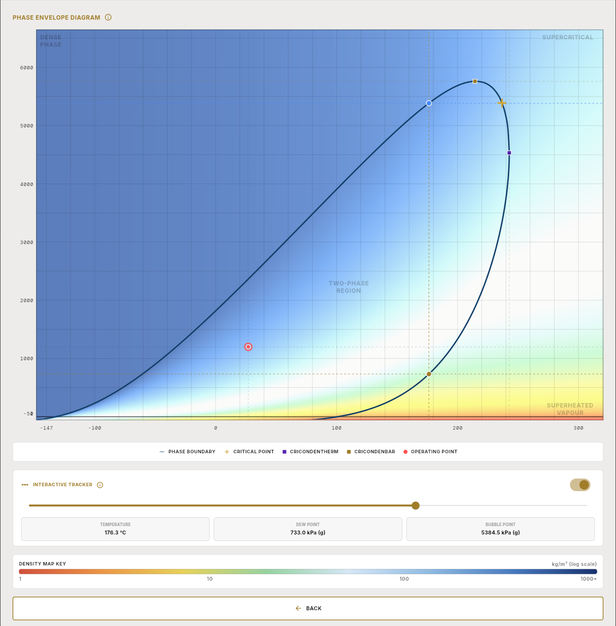
Phase Boundary & Density Solver's phase envelope diagram for the Gippsland Condensate stream: the traced phase boundary, critical point, cricondentherm, cricondenbar, and operating point at 1200.00 kPa(g) / 27.00°C, on a log-scale density map.

Captured from a single run of the app. The engine’s systematic checks against published reference data are reported on Validation & Verification.